Chapter 2 Discrete Planning
Chapter 2 Discrete Planning
2.1 Introduction to Discrete Feasible Planning
2.1.1 Problem Formulation
Formulation 2.1
State:
State space: , nonempty, finite or infinite.
Action:
Action space: ,
State transition fuction: . Each current state x, when applied with each action u, produces a new state x'.
Initial state:
Goal state:
2.1.2 Examples of Discrete Planning
- Moving on a 2D gird
Suppose that a robot moves on a grid in which each grid point has integer coordinates of the form (i, j). The robot takes discrete steps in one of four directions (up, down, left, right), each of which increments or decrements one coordinate. The motions and corresponding state transition graph are shown in Figure 2.1, which can be imagined as stepping from tile to tile on an infinite tile floor. This will be expressed using Formulation 2.1. Let X be the set of all integer pairs of the form , in which (Z denotes the set of all integers). Let . Let . The state transition equation is , in which and are treated as two-dimensional vectors for the purpose of addition. For example, if x = (3, 4) and u = (0, 1), then f (x, u) = (3, 5). Suppose for convenience that the initial state is . Many interesting goal sets are possible. Suppose, for example, that . It is easy to find a sequence of actions that transforms the state from (0, 0) to (100, 100).
- Rubik's Cube Puzzle
2.2 Searching for Feasible Plans
The methods presented in this section are just graph search algorithms, but with the understanding that the state transition graph is revealed incrementally through the application of actions, instead of being fully specified in advance.
An important point is that the search algorithms must be systematic, that is, the algorithm must keep track of states already visited.
2.2.1 General Forward Search
The following figure gives a general template of search algorithms. At any point during the search, there will be three kinds of states:
Unvisited: States that have not been visited yet. Initially, this is every state except xI.
Dead: States that have been visited, and for which every possible next state has also been visited. A next state of is a state for which there exists a such that In a sense, these states are dead because there is nothing more that they can contribute to the search. In some circumstances, of course, dead state can become alive again.
Alive: States that have been encountered, but possibly have unvisited next states. These are considered alive. Initially, the only alive state is .
Forward Search
Q.insert(x_I) and mark x_I as visited.

while Q not empty do:

     x = Q.GetFirst()

      if x in x_G:

        return SUCCESS

    for all u in U(x):

        x' = f(x,u)

          if x' not visited:

             Q.insert(x')

              mark x' visited

          else:

              Resolve duplicate x'

Return FAILURE
The above is a general template of forward search algorithm. Two focuses are presented here: How efficient is the test to determine whether in line 4? How can one tell whether has been visited in line 8 and line 9?
2.2.2 Particular Forward Search Methods
This section presents several search algorithms, each of which constructs a search tree. Each search algorithm is a special case of the algorithm of the forward search algorithm template demonstrated before, obtained by defining a different sorting function for Q. Most of these are just classical graph search algorithms.
Breath First: Specify Q as a First-In First-Out (FIFO) queue. All plans that have k steps are exhausted before plans with k + 1 steps are investigated. Therefore, breadth first guarantees that the first solution found will use the smallest number of steps. The asymptotic running time of breadth-first search is .
Depth First: Specify Q as a First-In Last-Out (FILO) stack. The running time of depth first search is also .
Dijkstra’s algorithm: Use cost-to-come (distance between initial state and current state), short for Function C, to sort Q.
A*: Incorporate a heuristic estimate of the cost called cost-to-go (distance between current state and goal state), short for with .
Best first: Only use to sort Q.
Iterative deepening: An approach integrates Breath first and Depth first method. That means performs Depth first search at i depth (i=1, 2, 3....max depth). Initially, i is equal to 1 and will increase with step going on. For example, if i = 1, the algorithm cannot find . Then i will be 2, perform the same operation. If we still cannot find the solution, i will be 3 until we reach .
2.2.3 Other General Search Schemes
- Backward search: For many planning problems, it might be the case that the branching factor is large when starting from xI. In this case, it might be more efficient to start the search at a goal state and work backward until the initial state is encountered.
BACKWARD SEARCH
Q.insert(x_G) and mark x_G as visited.
while Q not empty do:
x = Q.GetFirst()

if x in xI:

    return SUCCESS

for all u^-1 in U(x)^-1:

    x' = f^-1(x,u^-1)

    if x' not visited:

        Q.insert(x')

        mark x' visited

    else:

        Resolve duplicate x'
Return FAILURE
- Bidirectional search: One tree is grown from the initial state, and the other is grown from the goal state. The search terminates with success when the two trees meet. Failure occurs if either priority queue has been exhausted.
BIDIRECTIONAL SEARCH
Q_G.insert(X_G) and mark x_G as visited.

Q_I.insert(X_I) and mark x_I as visited.

while Q_G and Q_I not empty do:

    x = Q_I.GetFirst()

    if x already visited from x_G

        return SUCCESS

    for all u in U(x):

        x' = f(x,u)

        if x' not visited:

            Q_I.insert(x')

            mark x' visited

        else:

           Resolve duplicate x'

      x = Q_G.GetFirst()

   if x already visited from x_I

        return SUCCESS

   for all u^-1 in U(x)^-1:

        x' = f^-1(x,u^-1)

        if x' not visited:

           x_G.insert(x')

            mark x' visited

       else:

           Resolve duplicate x'

Return FAILURE
2.2.4 A Unified View of the Search Methods
For all search methods, there usually involves the following 6 steps:
Initialization: Initial graph G(V, E) and include some starting states in empty V, which could be or (Bidirectional search or backward search)
Select Vertex: Select states in priority queue Q sorted with some rules.
Apply an Action: Obtain a new state x' from f(x, u).
Insert a Directed Edge into the Graph: If certain algorithm-specific tests are passed, then generate an edge from x to x' for the forward case or an edge from xnew to x for the backward case. If x' is not yet in V , it will be inserted into V.
Check for Solution: Determine whether G encodes a path from to . If there is a single search tree, then this is trivial. If there are two or more search trees, then this step could be expensive.
Return to Step 2: Iterate unless a solution has been found or an early termination condition is satisfied, in which case the algorithm reports failure.
2.3 Discrete Optimal Planning
This section discusses optimal planning problems involving optimizing time, distance, energy consumed.
Formulation 2.2(Discrete Fixed-Length Optimal Planning)
All of the components from Formulation 2.1 will be inherited in this section like . Notably, here is finite.
The number of the stages, K, is defined, which is the exact length of the plan. It can be measured as the number of the actions. is obtained after is applied.
Introduce cost functional:
denote a stage-additive cost (or loss) functional, which is applied to a K-step plan, . This means that the sequence of actions and the sequence of states may appear in an expression of L.
For convenience, let F denote the final stage, (the application of advances the stage to )
The cost term yields a real value for every .
The final term is outside of the sum and is defined as if , and otherwise.
Distinguish
is the cost term after applying at while is the state transition fuction to obtain
2.3.1 Optimal Fixed-Length Plans
This section will mainly discuss the value iteration algorithm, which is to iteratively compute optimal cost-to-go (or cost-to-come) functions over the state space. In some conditions, it can be reduced to Dijkstra algorithm. There are mainly two versions of this algorithm, namely backward value iteration and forward value iteration.
2.3.1.1 Backward value iteration
Firstly, we will introduce a new cost fuctional called , which represents the cost accumulated through stage k to F. It can be written as the following equation:
This can be converted to the following equation (the proof process is omitted here as the formula will be well understood from its definition):
This produces the recurrence, which can be used to obtain iteratively from . It's like:
may contain the .
**Example**
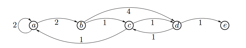
Suppose that . Hence, there will be four iterations by constructing .
Firstly, , For state a, b, c, e, they are not in , so each value of them is . For state d, the value is 0.
, can be a, b, c, d, e. Let's assume a as the current state()for instance. , the equation goes to . Here, . is the edge from a to . We need to find out the smallest of the five combinations of and . Obviously, all of them is .
Let's take b, c as the , respectively. You can see that . .
, the potential options of . You need to take a,b,c,d,e as to calculate their optimal value . For example, d as . There are five circumstances, in which 3 of them are (a, d, e). So the left two are . So .
In this way can you easily obtain . The results are shown in the following table.
| a | b | c | d | e | |
|---|---|---|---|---|---|
| G₅* | ∞ | ∞ | ∞ | 0 | ∞ |
| G₄* | ∞ | 4 | 1 | ∞ | ∞ |
| G₃* | 6 | 2 | ∞ | 2 | ∞ |
| G₂* | 4 | 6 | 3 | ∞ | ∞ |
| G₁* | 6 | 4 | 5 | 4 | ∞ |