改进NS模型

本节介绍NS模型基本内容、改进NS模型以及对应代码的实现。

1 基本概念

1.1 Nagel–Schreckenberg model NS模型

Nagel–Schreckenberg model，简称NS model，最初由德国物理学家Kai Nagel and Michael Schreckenberg,是一种基于CA模型的用于交通仿真的理论模型。

Nagel–Schreckenberg model, short for NS model, first develped by German physicists Kai Nagel and Michael Schreckenberg, is a theoretical Cellular Automata-based model for traffic simulation.

1.2 Rule 184

补充一下基于CA交通仿真中最常见的规则，即 Rule 184，即对于一条道路上连续的三个cell，他们的状态有以下8种（用0代表空，用1代表有车占有）,如下图所示：

Rule 184

1.3 Phantom traffic jam 幽灵拥堵

• 定义：莫名发生的交通拥堵 traffic jam without clear reasons

• 原因：在拥堵（heavy）交通流中，微小的交通扰动（small disturbances），如司机过度刹车或者与其他车里的太近，都会被放大形成(be amplified into)内生性的交通拥堵。 Small disturbances, such as overreations of braking or getting too close to another vehicle, in heavy traffic can be amplified into a self-sustained traffic jam.

• 结果：形成stop-and-go wave

Stop-And-Go Wave

字面意是停走波

形成原因：

• 微观（从driver角度）：vehicle slowly move → decelerate → stop → accelerate →
• 宏观，如下图Time-Space Diagram所示：

Time-Space Diagram 时空图

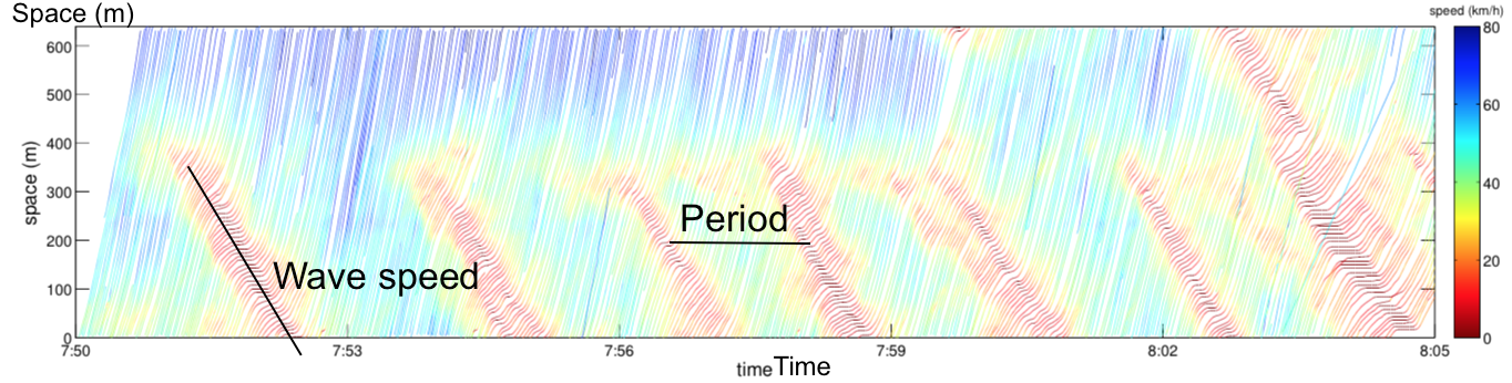
由上图可以看到stop-and-go wave沿车流末端传播的速度，即wave speed以及波次间隔时间wave period。

这样的stop-and-go wave会造成以下危害：

• 更费油与更多排放 more fuels and emmisions.
• 更加危险 more dangerous.

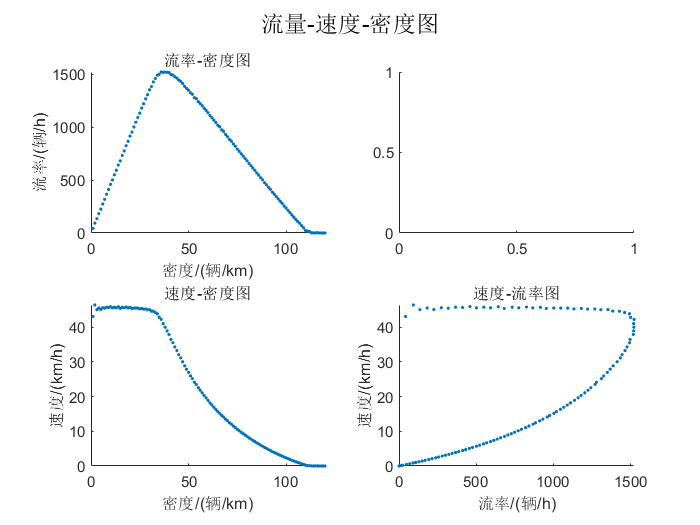
1.4 基本图 Fundamental Diagram

Fundamental Diagram 基本图

• Capacity/Maximum Flow 极大流率：qk曲线极值
• Free Flow Speed 畅行速度：k=0对应的速度
• Critical Density 临界密度：极大流率对应的密度
• Critical Speed 临界速度：极大流率对应的速度
• Jam Density 堵塞密度：v=0时的密度

2 Model Description 模型描述

2.1 Model Information 模型说明

• 空间时间上均离散化。 Discrete in space and time

• 所有车辆同步更新。 Each vehicle is updated parallel

• 每个元胞长7.5m（包括了车长+距离前车的安全距离）。 Lane is divided into cells of length 7.5 m, which includes the vehicle length and the safe distance to the preceeding/leading vehicle.

• 每个元胞为空或仅被一辆车占据。 Each cell can either be empty or occupied by only one vehicle.

• 每个车辆拥有坐标、速度属性，车辆有最大速度限制。 Each vehicle is characterized by its velocity and coordinates. The velocity has a limit.

2.2 Model Step 更新规则

• Step 1：加速 Acceleration：对于未到达最大速度的车辆，以一个单位加速。 For vehicle not reaching speed limit, it accelerates with 1 unit.

$$v(i) \rightarrow \min{v(i) + 1, V_{\text{max}}}$$

这反应了司机希望开得越快越好 reflect the desire of drivers to drive as fast as possible.

• Step 2: 减速 Safe Distance Judgment：当汽车当前速度大于与前车的距离（前方的空元胞数），则汽车减速为安全距离，否则维持原速。
  If vehicle speed is larger than the number of empty cells in front of it, it velocity reduces to that empty cell amount. Otherwise, it keeps its speed.

$$v(i) \rightarrow \min{v(i) , d(i)}$$

It encodes the interaction between the vehicle. In this simple model, interactions only occur to avoid collision.

• Step 3：随机慢化 Randomization：车辆以p的概率随机减速一个单位，p称为随机慢化概率。 The speed of vehicle reduces by one unit with slowdown probability p.

$${v(i) \rightarrow \max{v(i) - 1, 0}}$$

反映驾驶员的不完美驾驶行为（imperfect behavior of drivers），比如在步骤2减速时刹车踩的过大。在现实场景，驾驶员不可能总是按照一定速度(constant speed)行驶，总会有一定的波动(fluctuations)。当车流量足够大，驾驶员的这一行为会引起交通系统的一系列反应，最终形成拥堵现象。这也是反映了拥堵总是在没有任何外部原因（external reasons ，如事故）就会发生的，因此称为幽灵拥堵（phantom jam）。

Randomization reflects the imperfect behavior of drivers like the overreations of braking in Step 2. In real-world scenario, drivers cannot always drive at a constant speed. There always has fluctuations of the velocity.

• Step 4: 位置更新 Driving：每个车辆前进当前速度的格数。 Every vehicle forward by v(i) cells.

3 改进NS模型 NS Model for Inhomogenous Traffic Flow in a Single Lane

3.1 改进点：

1. 车辆以最大加速度 $a_{max}$ 加减速而不是以1 Vehicle accelerates/decelerates with maximum acceleration not 1.
2. 引入慢启动系数s（反应静止车辆启动较慢） Introduce the Slow Start probability(short for s) to reflect the difficuty of stationary vehicles to start up.
3. 考虑异质(inhomogeneous)车流（反映在车长，最大速度，最大加速度） Consider the inhomogeneous flow like the vehicle length, maximum velocity and maximum acceleration.

3.2 模型信息

单车道 周期边界 Single Lane with Periodic Boundary

模型信息

3.3 结果

通过改变货车占比r(propotion of trucks)、随机慢化概率p以及慢启动系数s，分别做FD图以及时空位置图，分别分析其对于交通系统的影响影响。

如当s = 0.1, p = 0.3 条件下，分别做r=0,0.1,0.2,0.3的时空位置图(Time-Space Diagram)以及基本图（Fundemantal Diagram, FD）,红线为货车，黑线为小汽车。

r=0

r=0.1

r=0.2

r=0.3

r=0 含速度

r=0.1 含速度

r=0.2 含速度

r=0.3 含速度

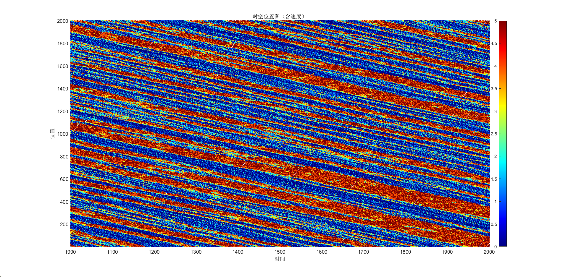
可以看到随着货车比例的增加，wave speed逐渐降低，wave period也逐渐变小，反应交通系统越来越拥堵。

做FD图如下：

r=0

r=0.1

r=0.2

r=0.3

r	极大流率Qm	临界密度Kc	临界速度Vc	堵塞密度Kj	畅行速度Vf
0	2326.9176	19	122.4693	140	126.7668
0.01	1782.0972	40	44.5524	138	126.8262
0.03	1702.6758	40	42.5669	131	126.9054
0.05	1647.4248	39	42.2417	127	46.3035
0.1	1534.3903	37	43.0448	115	46.4292
0.2	1377.4356	34	40.5128	99	46.0799
0.3	1241.7444	32	38.8045	86	42.9739

随着货车比例r的增加，Qm逐渐减小，Kc先增加后减小，Vc先急剧减小后基本不变，Kj逐渐减小，Vf先不变后急剧减小。

通过改变s与p的大小，也可以同理做出上述图表，这里不一一展示。

3.4 代码

完整代码，内含动画演示。

3.5 进一步的改进点

• 多车道，考虑换道，如STCA模型。
• Velocity-Dependent-Randomization（VDR）：NS模型中p是固定不变的，VDR中p是v的函数（与加入随机慢化概率s效果类似）。

STCA（[以下内容源于][m]）

由Rickert M和Chowdhury D等人在单车道元胞自动机Nasch模型的基础上提出了双车道元胞自动机STCA模型。该模型将模拟的道路环境扩展为双车道，增加了车辆换道规则，使之能够更真实准确地模拟出道路上交通流的运行状况。

STCA模型在应用过程中将一个时步分为两个相同的子时步。第一个时步为车辆换道时步，车辆在这个时步内按照设计的换道规则决定是否发生换道行为；第二个时步为演化更新时步，两条车道上的车辆在该时步均按照单车道元胞自动机模型中设计的演化更新规则运行。

换道规则一般包括两个部分：

1. 换道动机： 换道动机是指驾驶员想换道的意愿和条件。当某车辆在当前车道上无法达到驾驶员的期望速度，而另一条车道上的驾驶条件可以满足驾驶员对速度的要求时，车辆会以一定的换道概率进行换道。

$$\begin{array}{r} d_n<\Delta t \min \left(v_n+1, v_{\max }\right) \\ d_{n, \text { sidefront }}>d_n \cdots \end{array}$$

2. 安全条件： 安全条件是指车辆在决定换道时要确定当前交通状况下换道对于自身和其他车辆是否安全，避免因车辆换道引起交通事故，危害生命财产安全。

$$d_{n, \text { sideback }}>d_{\text {safe }}$$